The allocation of decision rights in a firm creates a problem, as the interests of the owners and employees are not always aligned. This is known as the principal-agent problem.
Principal-agent problems are typically modelled as a game between two players, the principal and the agent, who face a conflict of interest. In the case of an employer and employee, the employer is the principal and the employee the agent. The misalignment of interests creates a challenge in designing incentives to align those interests.
Below, I examine two classes of principal-agent problem.
The first is where the agent’s action is observable by the principal. Consider a production line, where the employee has a discrete task to complete. The employer can observe exactly how hard they are working via the number of items they produce.
I will show that incentive conflicts do not cause problems when effort is observable, enabling a contract to be developed. The employer can simply specify the appropriate level of effort for which a bonus is payable.
However, outside of idealised problems, an agent’s effort is not usually costlessly observable by the firm. They can’t simply contract to deliver a set amount of effort. Further, output may not reflect effort. There are likely other effects on output besides the agent’s effort. In addition, other proxies for effort might be difficult to measure.
Consider an employee whose role is risk management on the production line. Their activities might include checking the quality of the products, developing safety policies, liaising with management and dealing with unexpected events. The firm can’t observe the effort that goes into these tasks.
Therefore, a second class of principal-agent problem involves hidden actions, where the conflict between the principal and the agent is over an action the agent may take, and this action cannot be detailed in a complete contract. The agent knows what action is taken, but the principal doesn’t. For our employer-employee problem, the hidden action is the employee’s effort. There is a problem because the employer would like the employee to work hard, whereas the employee would prefer to take it easy.
To illustrate the principal-agent problem, below are illustrations of this challenge with observable and unobservable effort. In each case, I provide one narrative and one mathematical description of the problem. The following are based on examples in Brickley et al. (2020).
5.1 Observable effort
5.1.1 A narrative exploration
The owner of ACME Corporation wants their employees to put in higher effort and work diligently. However, their employee Ian, while liking to be paid, doesn’t like to put in effort. As Ian’s income goes up, he is happier, but he is also happier the more he can lounge around in the office and cruise Facebook.
Ian won’t get out of bed and turn up to work for less than $1,000 a week. That is what we call his reservation wage. He then needs to be paid for his efforts in the office. He has a mentally taxing job, so each hour of effort is harder than the last. As a result, he will demand a salary of at least $1000 plus a compensating amount for whatever level of effort he provides.
The firm benefits from Ian’s effort, receiving around $100 for every hour he applies himself.
If the firm could tell whether Ian was working or not, they could just agree on a level of effort, pay him an agreed sum for it, and then monitor to make sure he delivers. What is that sum?
The firm will want to pay Ian the sum that maximises its profit. Ian wants to set his level of effort to balance his desire for income and the increasing cost of effort. As the firm receives $100 for every hour he works, they will pay Ian up to the point where he demands more than $100 for each additional hour.
In classical economic terms, the marginal benefit to the firm of each hour that Ian works is $100. Their profit will be maximised when that marginal benefit is equal to the marginal cost of inducing an additional hour of effort from Ian. The firm could pay him more to get even more effort and output, but the cost of inducing this effort would exceed the benefit they receive.
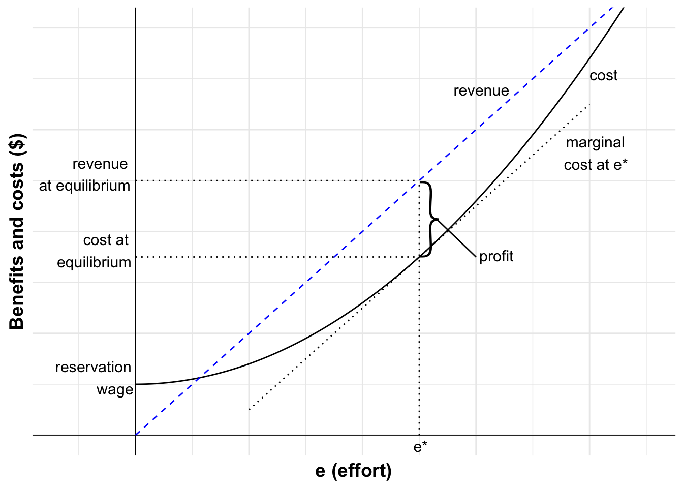
Here is the problem illustrated graphically.
On the horizontal axis is the amount of effort expended by Ian. The costs and benefits of Ian’s effort are on the vertical axis.
The dashed blue line represents the increasing benefit from each hour of effort. Each additional hour of effort delivers $100 extra benefit to the firm.
The curved black line represents the cost of effort to Ian. Each additional hour of effort is harder to deliver than the last, so Ian’s cost is increasing in the amount of effort.
Code
library(ggplot2)# Function definitionscost <-function(x){1000+x^(2)}revenue <-function(x){100*x}# Create a data frame with effort and cost datadf <-data.frame(x=seq(0,100,0.1),y=NA)df$y <-cost(df$x)#Variables for plotestar<-50#equilibrium effort# Create base plot with common elementscreate_base_plot <-function(data) {ggplot(mapping =aes(x, y)) +# Plot the effort cost curvegeom_line(data = data) +geom_vline(xintercept =0, linewidth =0.25) +geom_hline(yintercept =0, linewidth =0.25) +labs(x ="e (effort)", y ="Benefits and costs ($)") +# Set the themetheme_minimal() +# Remove numbers on each axistheme(axis.text.x =element_blank(),axis.text.y =element_blank(),axis.title =element_text(size =14, face ="bold"),axis.title.y =element_text(angle =90, vjust =0.5)) +# Limit to y greater than zero and x greater than -8coord_cartesian(xlim =c(-13, 90), ylim =c(0, 8000)) +# Set grid lines spaced by 20scale_x_continuous(breaks =seq(0, 100, by =20))}paPlot <-create_base_plot(df) +#Add the revenue line starting at the origingeom_segment(aes(x =0, y =0, xend =100, yend =10000), linetype ="dashed", color ="blue")+#add label to revenue lineannotate("text", x =60, y =6700, label ="revenue", size =4, color ="blue")+#add label to cost lineannotate("text", x =82, y =7200, label ="cost", size =4)+#add a tangent to the cost curve at e* and a label "marginal cost"annotate("segment", x =20, xend =80, y =500, yend =6500, linewidth =0.5, colour ="black", linetype="dotted")+annotate("text", x =80, y =5500, label ="marginal\ncost at e*", size =4)#create version without numbers on axespaPlot+#add label for reservation wage where cost curve intercepts y-axisannotate("text", x =-8, y =1000, label ="reservation\nwage", size =4)+#Add line indicating cost and revenue of equilibrium effort, including labelsannotate("segment", x =0, y =cost(estar), xend = estar, yend =cost(estar), linewidth =0.5, colour ="black", linetype="dotted")+annotate("text", x =-8, y =cost(estar), label ="cost at \n equilibrium", size =4)+annotate("segment", x =0, y =revenue(estar), xend = estar, yend =revenue(estar), linewidth =0.5, colour ="black", linetype="dotted")+annotate("text", x =-9, y =revenue(estar), label ="revenue \n at equilibrium", size =4)+#Add vertical line indicating equilibrium effort and labelled "e*"annotate("segment", x = estar, xend = estar, y =0, yend =revenue(estar), linewidth =0.5, colour ="black", linetype="dotted")+annotate("text", x = estar, y =-200, label ="e*", size =4)+#add curly bracket indicating profit at e* between revenue and cost lines, and a line to the label "profit"annotate("text", x =52, y =4150, label ='{', angle =180, size =23, family ='Source Sans Pro ExtraLight')+annotate("segment", x =53, xend =60, y =4250, yend =3500, linewidth =0.5, colour ="black")+annotate("text", x =63, y =3550, label ="profit", size =4)
Figure 5.1: Maximising profit with observable effort
From the firm’s perspective, for any level of effort, they gain the benefit of $100 per hour expended. They have to pay the cost of Ian expending the effort. As a profit-maximising firm, they will achieve their objective where the gap between cost and benefit is maximised.
Visually, you can see this point on the chart where the gap between the two lines is largest. What you might notice is that, at this point, the two lines are parallel to each other. They have the same slope. This indicates that the marginal benefit of the effort - the amount the firm gets for one additional unit of effort at this point - equals the marginal cost of the effort - the amount that the employee demands for expending one additional unit of effort.
If Ian were paid for another hour of effort over the optimal level, he would demand more than $100, reducing the firm’s profit, as the firm receives only $100 for that additional hour of effort. Conversely, the firm’s profit would decline if Ian were paid for one hour less effort. At that point, Ian demands less than $100 per hour for each unit of effort, meaning the firm could gain by paying for the hour and receiving the $100 of output.
5.1.2 A mathematical exploration
Ian’s utility (U) is a function of his income (W) and his effort (e, the hours actually spent working). Utility is increasing in income (+ve) and decreasing (-ve) in effort. Let:
U(W,e)=W-e^2
Ian’s reservation wage is $1,000.
The firm gets $100 of output for every hour Agent A works:
Q=\$100e
Assume that effort is observable at zero cost and verifiable. It is possible to contract over effort. In this case, the firm will offer Ian a contract requiring he put in a specified level of effort e^*.
The contract will be acceptable to Ian if he receives at least their reservation level of utility. That is, the contract will be acceptable as long as it pays:
W=\$(1000+(e^*)^2)
If Ian accepts the contract, he gets utility:
U(.)=1000+(e^*)^2-(e^*)^2=1000
The firm’s challenge is to maximise profit (\pi). That is:
To determine the level of effort, we take the first order derivative of the profit function with respect to effort. We then set this first order condition to zero:
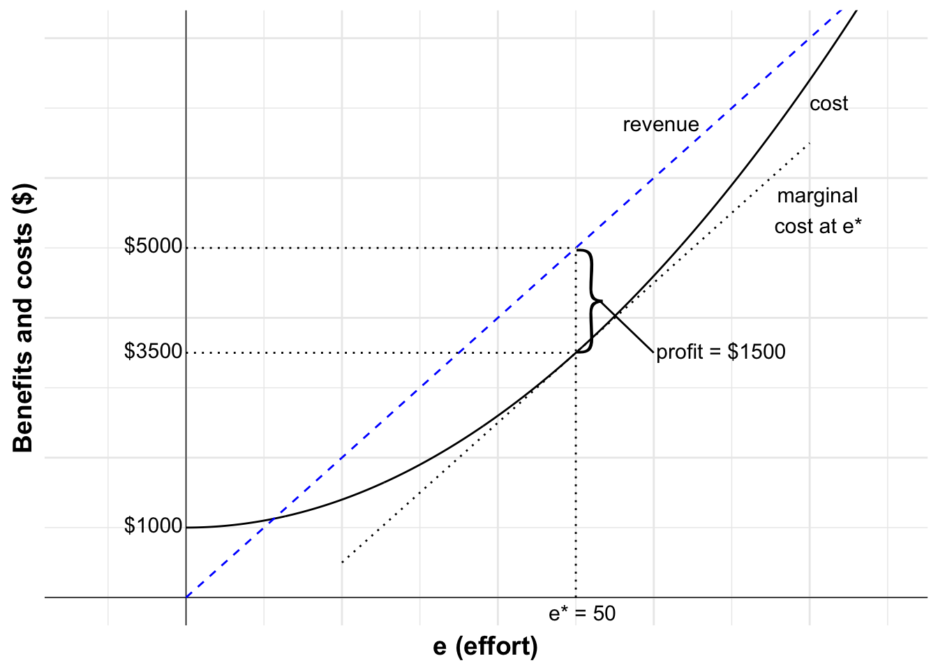
These numerical answers can be seen in the diagram.
At effort level e^*=50, the marginal benefit of effort is equal to the marginal cost of inducing effort. At that level of effort, Ian receives $3500 in compensation. The firm receives $5000 in revenue. The firm’s profit is their revenue minus the cost, being $1500.
Code
#create version with numbers instead of labelspaPlot+#add label for reservation wage where cost curve intercepts y-axisannotate("text", x =-4, y =1000, label ="$1000", size =4)+#Add line indicating cost and revenue of equilibrium effort, including labelsannotate("segment", x =0, y =cost(estar), xend = estar, yend =cost(estar), linewidth =0.5, colour ="black", linetype="dotted")+annotate("text", x =-4, y =cost(estar), label ="$3500", size =4)+annotate("segment", x =0, y =revenue(estar), xend = estar, yend =revenue(estar), linewidth =0.5, colour ="black", linetype="dotted")+annotate("text", x =-4, y =revenue(estar), label ="$5000", size =4)+#Add vertical line indicating equilibrium effort and labelled "e*"annotate("segment", x = estar, xend = estar, y =0, yend =revenue(estar), linewidth =0.5, colour ="black", linetype="dotted")+annotate("text", x = estar, y =-200, label ="e* = 50", size =4)+#add curly bracket indicating profit at e* between revenue and cost lines, and a line to the label "profit"annotate("text", x =52, y =4150, label ='{', angle =180, size =23, family ='Source Sans Pro ExtraLight')+annotate("segment", x =53, xend =60, y =4250, yend =3500, linewidth =0.5, colour ="black")+annotate("text", x =68.5, y =3550, label ="profit = $1500", size =4)
Figure 5.2: Maximising profit with observable effort: numerical example
5.2 Unobservable effort
5.2.1 A narrative exploration
Erica is a risk-neutral employee of Acme Corporation. If the firm could observe Erica’s effort, the firm could simply develop a contract under which Erica is paid for a set level of effort. However, Erica’s effort is unobservable in that the firm cannot, at any point, see how much effort she is putting in.
Erica’s output increases with her effort. This might suggest the firm could simply contract for a set amount of output. However, for this example, Erica’s output is subject to other random effects outside her control.
Therefore, paying Erica a fixed salary to deliver a set level of effort or output is problematic. She could blame the low output on bad luck.
An alternative is for the firm to pay Erica a fixed sum plus a share of her output. This is feasible if the random effects and Erica’s effort are independent. As long as the output and associated compensation increase with every unit of Erica’s effort, she will not need to consider the effects on output that are out of her control.
Erica will want to be compensated for her effort. She will set her effort level such that her expected compensation minus the cost of the effort is maximised. This is at the level of effort where the marginal benefit of increased compensation equals the marginal cost of additional effort.
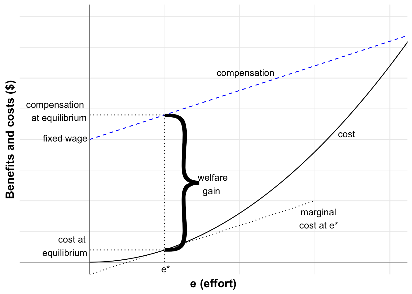
Here is the scenario illustrated graphically.
On the horizontal axis is the amount of effort expended by Erica. The costs and benefits of Erica’s effort are on the vertical axis.
Code
# Define the cost and compensation functionscost_erica <-function(x) { x^(2)}compensation <-function(x) {1000+20* x}# Create a data frame with the x variabledf_erica <-data.frame(x =seq(0, 50, 0.1),y =cost_erica(seq(0, 50, 0.1)))# Variables for plot (may not match labels as not done to scale)# Payoffs from gambleestar <-10# equilibrium effort# Create the plotericaPlot <-ggplot(mapping =aes(x, y)) +# Plot the effort cost curvegeom_line(data = df_erica) +geom_vline(xintercept =0, linewidth =0.25) +geom_hline(yintercept =0, linewidth =0.25) +labs(x ="e (effort)", y ="Benefits and costs ($)") +# Add the compensation line starting at the base paygeom_segment(aes(x =0, y =1000, xend =50, yend =compensation(50)), linetype ="dashed", color ="blue") +# Set the themetheme_minimal() +# Remove numbers on each axistheme(axis.text.x =element_blank(),axis.text.y =element_blank(),axis.title =element_text(size =14, face ="bold"),axis.title.y =element_text(angle =90, vjust =0.5)) +# Add label to cost lineannotate("text", x =35, y =1100, label ="cost", size =4) +# Limit to y greater than zero and x greater than -8 (need -8 so space for y-axis labels)coord_cartesian(xlim =c(-7, 40), ylim =c(0, 2000)) +# Set grid lines spaced by 10scale_x_continuous(breaks =seq(0, 100, by =20))# Create version without numbers on axesericaPlot2 <- ericaPlot +# Add label for reservation wage where cost curve intercepts y-axisannotate("text", x =-3.5, y =compensation(0), label ="fixed wage", size =4) +# Add line indicating cost and revenue of equilibrium effort, including labelsannotate("segment", x =0, y =cost_erica(estar), xend = estar, yend =cost_erica(estar), linewidth =0.5, colour ="black", linetype ="dotted") +annotate("segment", x =0, y =compensation(estar), xend = estar, yend =compensation(estar), linewidth =0.5, colour ="black", linetype ="dotted") +# Add vertical line indicating equilibrium effort and labelled "e*"annotate("segment", x = estar, xend = estar, y =0, yend =compensation(estar), linewidth =0.5, colour ="black", linetype ="dotted") +annotate("text", x = estar, y =-50, label ="e*", size =4) +# Add a tangent to the cost curve at e* and a label "marginal cost"annotate("segment", x =0, xend =30, y =-100, yend =500, linewidth =0.5, colour ="black", linetype ="dotted") +annotate("text", x =33, y =520, label ="marginal\ncost at e*", size =4)ericaPlot2 +# Add vertical lines with arrows to indicate welfare gaingeom_segment(aes(x = estar, xend = estar, y =cost_erica(estar), yend =compensation(estar)), colour ="black", linetype ="dashed", arrow =arrow(type ="closed", length =unit(0.15, "inches"))) +geom_segment(aes(x = estar, xend = estar, y =compensation(estar), yend =cost_erica(estar)), colour ="black", linetype ="dashed", arrow =arrow(type ="closed", length =unit(0.15, "inches"))) +annotate("text", x = estar +3.7, y = (cost_erica(estar) +compensation(estar)) /2, label ="welfare gain", size =4, colour ="black") +# Add line indicating new compensation equilibrium plus labels for new higher equilibrium compensationannotate("text", x =-4, y =compensation(estar), label ="compensation \n at equilibrium", size =4)+# Add label to compensation lineannotate("text", x =20, y =1550, label ="compensation", size =4, color ="blue")+# Add line and label for cost at equilibriumannotate("text", x =-3.5, y =cost_erica(estar), label ="cost at \n equilibrium", size =4)
Figure 5.3: Erica’s optimal effort when unobservable
This dashed blue line represents Erica’s compensation, which comprises a fixed sum payment plus the increasing wage from her share of the output. Suppose the firm gains $100 of output from each unit of unobserved effort and is willing to pay Erica a 20% share. Therefore, each additional unit of effort delivers Erica $20.
The curved black line represents the cost of effort to Erica. Each additional hour of effort is harder to deliver than the last, so Erica’s cost is increasing in the amount of effort.
Erica maximises her utility at the point where the gap between her compensation and cost of effort is the greatest. Visually, you can see this point on the chart where the gap between the two lines is largest. At this point, the two lines are parallel to each other. They have the same slope. This indicates that the marginal benefit of Erica’s effort - the amount Erica gets for investing one additional unit of effort - equals the marginal cost of the effort - the cost Erica incurs for expending one additional unit of effort.
As Erica’s effort and the random shocks are independent, the marginal cost and benefit of effort are not affected by the random shocks that otherwise affect her payment. A random effect that reduces output does not change the fact that extra effort increases output and, accordingly, Erica’s compensation.
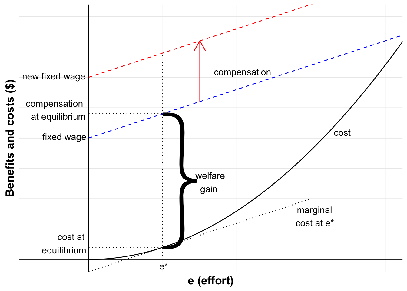
5.2.1.1 Increasing the fixed wage
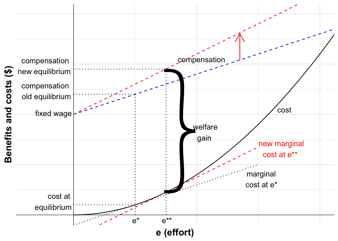
Suppose the firm decided to increase the fixed portion of Erica’s wage. This has the effect of moving the compensation line in the diagram upwards. Although this increases Erica’s income for any specific level of effort, this does not change the incentives for Erica, as the marginal benefit and cost remain equal at the same level of effort. She will apply the same level of effort regardless of the fixed wage change. As a result, the firm’s profit would drop.
Code
ericaPlot2+#Add label for cost at equilibriumannotate("text", x =-3.5, y =cost_erica(estar), label ="cost at \n equilibrium", size =4)+#Add the compensation line starting at the base paygeom_segment(aes(x =0, y =1500, xend =100, yend =3500), linetype ="dashed", color ="red")+#Add vertical line indicating equilibirum stays the sameannotate("segment", x = estar, xend = estar, y =0, yend =compensation(estar)+500, linewidth =0.5, colour ="black", linetype="dotted")+#Add red vertical line with arrow between the two compensation lines indicating increaseannotate("segment", x =15, xend =15, y =compensation(15), yend =compensation(15)+500, arrow =arrow(type ="open", angle =30, length =unit(0.5, "centimeters")), colour ="red")+#add label for new higher fixed wageannotate("text", x =-4.7, y =1500, label ="new fixed wage", size =4)+#add vertical lines with arrows to indicate welfare gaingeom_segment(aes(x = estar, xend = estar, y =cost_erica(estar), yend =compensation(estar)+500), colour ="black", linetype ="dashed", arrow =arrow(type ="closed", length =unit(0.15, "inches"))) +geom_segment(aes(x = estar, xend = estar, y =compensation(estar), yend =cost_erica(estar)), colour ="black", linetype ="dashed", arrow =arrow(type ="closed", length =unit(0.15, "inches"))) +annotate("text", x = estar +3.7, y = (cost_erica(estar) +compensation(estar)+500) /2, label ="welfare gain", size =4, colour ="black") +annotate("text", x =-4.5, y =compensation(estar), label ="compensation \n old equilibrium", size =4)+# add line and label for new equilibrium compensationannotate("segment", x =0, y =compensation(estar)+500, xend = estar, yend =compensation(estar)+500, linewidth =0.5, colour ="black", linetype="dotted")+annotate("text", x =-4.5, y =compensation(estar)+500, label ="compensation \n new equilibrium", size =4)+# Add label to compensation lineannotate("text", x =14, y =1900, label ="compensation", size =4, color ="red")
Figure 5.4: Increasing the fixed wage with unobservable effort
5.2.1.2 Increasing the share of output
The firm could, alternatively, increase the share of the output it pays to Erica. This increases the slope of the line for compensation. The marginal benefit of an extra unit of effort will now equal the marginal cost at a higher level of effort. Erica’s effort increases. Whether the firm is willing to do this depends on the profit-maximising level of effort and compensation.
Code
compensation3 <-function(x) {1000+30* x}ericaPlot2+#Add the compensation line with a slope of 0.3geom_segment(aes(x =0, y =1000, xend =100, yend =4000), linetype ="dashed", color ="red")+#add a tangent to the cost curve at e** and a label "new marginal cost"annotate("segment", x =0, xend =30, y =-225, yend =675, linewidth =0.5, colour ="red", linetype="dashed")+annotate("text", x =33, y =750, label ="new marginal\ncost at e**", size =4, color="red")+#Add vertical line at new higher equibrium effortannotate("segment", x =15, xend =15, y =0, yend =1450, linewidth =0.5, colour ="black", linetype="dotted")+annotate("text", x =15, y =0, label ="e**", size =4, hjust =0.4, vjust =1.5)+#Add red vertical line with arrow between the two compensation lines indicating increaseannotate("segment", x =27, xend =27, y =compensation(27), yend =compensation3(27), arrow =arrow(type ="open", angle =30, length =unit(0.5, "centimeters")), colour ="red")+#add vertical lines with arrows to indicate welfare gaingeom_segment(aes(x =15, xend =15, y =cost_erica(15), yend =compensation3(15)), colour ="black", linetype ="dashed", arrow =arrow(type ="closed", length =unit(0.15, "inches")))+geom_segment(aes(x =15, xend =15, y =compensation3(15), yend =cost_erica(15)), colour ="black", linetype ="dashed", arrow =arrow(type ="closed", length =unit(0.15, "inches")))+annotate("text", x =16, y = (cost_erica(15) +compensation3(15)) /2, label ="welfare gain", size =4, hjust =0.1, vjust =1.5, colour ="black")+# Add line indicating new compensation equilibrium plus labels for new higher equilibrium compensationannotate("segment", x =0, y =compensation3(15), xend =15, yend =1000+15*30, linewidth =0.5, colour ="black", linetype="dotted")+annotate("text", x =0, y =compensation(estar), label ="compensation \n old equilibrium", size =4, hjust =1.05, vjust =0.3)+annotate("text", x =0, y =compensation3(15), label ="compensation \n new equilibrium", size =4, hjust =1.05, vjust =0.3)+# Add label to compensation lineannotate("text", x =19, y =1750, label ="compensation", size =4, color ="red")+# add line and label for cost at old and new equilibriumannotate("segment", x =0, y =cost_erica(15)-10, xend =15, yend =cost_erica(15), linewidth =0.5, colour ="black", linetype="dotted")+annotate("text", x =-3.5, y =cost_erica(15)+70, label ="cost new \n equilibrium", size =4)+annotate("text", x =-3.5, y =cost_erica(estar), label ="cost old \n equilibrium", size =4)
Figure 5.5: Increasing the output share with unobservable effort
5.2.2 A mathematical exploration
Assume that we have a risk-neutral employer and a risk averse-employee, Erica, who has output given by the following:
Q=\alpha e+\mu \\[12pt]
\mu\sim(0,\sigma^2)
Q is the value of the output (which is observable); e is effort; \alpha is Erica’s marginal productivity, and \mu is some random effect.
If effort (e) could be observed, we might expect a contract that specifies a level of effort e^* for a fixed salary W.
That contract would deliver profit to the firm of:
\pi=(\alpha e+\mu)-W
But suppose neither e nor \mu is observable. The firm can’t pay her for a set level of effort. The firm also can’t pay her a fixed sum for a set production level, as Erica may put in low effort and blame the low output on bad luck (a low \mu).
However, the firm could incentivise Erica by basing her compensation on output. Consider her effort problem if she is paid according to the following linear payment schedule:
W=W_0+\beta Q \\[12pt]
\\
0\leq \beta \leq 1
where W_0 is a fixed wage and \beta is the proportion of output (Q) received.
This type of contract might represent a typical compensation scheme. Let W_0=1000 and \beta=0.2.
Solving this, Erica sets her level of effort where the compensation minus cost of effort is greatest. Note that an extra unit of effort always increases compensation by $20. The random component or shock (\mu) affects the total level of payment, but not the marginal impact of effort. This means that Erica can effectively ignore \mu.
We can calculate Erica’s optimal effort by taking the first derivative of her utility function, incorporating the compensation function and her cost of effort, and setting it to zero. We then solve for the effort level.
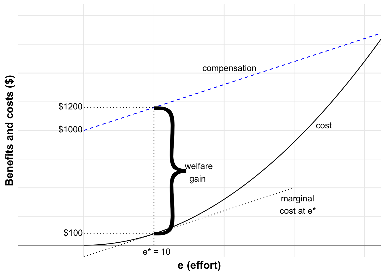
In this case, the optimal choice of effort is equal to 10. A plot illustrating this is shown below.
Code
#create version with numbersericaPlot3 <- ericaPlot+#add label for reservation wage where cost curve intercepts y-axisannotate("text", x =-2, y =1000, label ="$1000", size =4)+#Add line indicating cost and revenue of equilibrium effort, including labelsannotate("segment", x =0, y =cost_erica(estar), xend = estar, yend =cost_erica(estar), linewidth =0.5, colour ="black", linetype="dotted")+annotate("text", x =-2, y =cost_erica(estar), label ="$100", size =4)+annotate("segment", x =0, y =compensation(estar), xend = estar, yend =compensation(estar), linewidth =0.5, colour ="black", linetype="dotted")+annotate("text", x =-2, y =compensation(estar), label ="$1200", size =4)+#Add vertical line indicating equilibirum effort and labelled "e*"annotate("segment", x = estar, xend = estar, y =0, yend =compensation(estar), linewidth =0.5, colour ="black", linetype="dotted")+annotate("text", x = estar, y =0, label ="e* = 10", size =4, hjust =0.4, vjust =1.5)+#add a tangent to the cost curve at e* and a label "marginal cost"annotate("segment", x =0, xend =30, y =-100, yend =500, linewidth =0.5, colour ="black", linetype="dotted")+annotate("text", x =30, y =520, label ="marginal\ncost at e*", size =4, hjust =0.4, vjust =1.5)ericaPlot3+#add vertical lines with arrows to indicate welfare gaingeom_segment(aes(x = estar, xend = estar, y =cost_erica(estar), yend =compensation(estar)), colour ="black", linetype ="dashed", arrow =arrow(type ="closed", length =unit(0.15, "inches")))+geom_segment(aes(x = estar, xend = estar, y =compensation(estar), yend =cost_erica(estar)), colour ="black", linetype ="dashed", arrow =arrow(type ="closed", length =unit(0.15, "inches")))+annotate("text", x = estar +1, y = (cost_erica(estar) +compensation(estar)) /2, label ="welfare gain", size =4, hjust =0.1, vjust =1.5, colour ="black")+# Add label to compensation lineannotate("text", x =20, y =1550, label ="compensation", size =4, color ="blue")
Figure 5.6: Optimal effort with unobservable effort
5.2.2.1 Increasing the fixed wage
A change in W_0 doesn’t change incentives around effort. With a higher intercept, the optimal choice of effort is unchanged. What is important is the marginal benefit and marginal cost of effort.
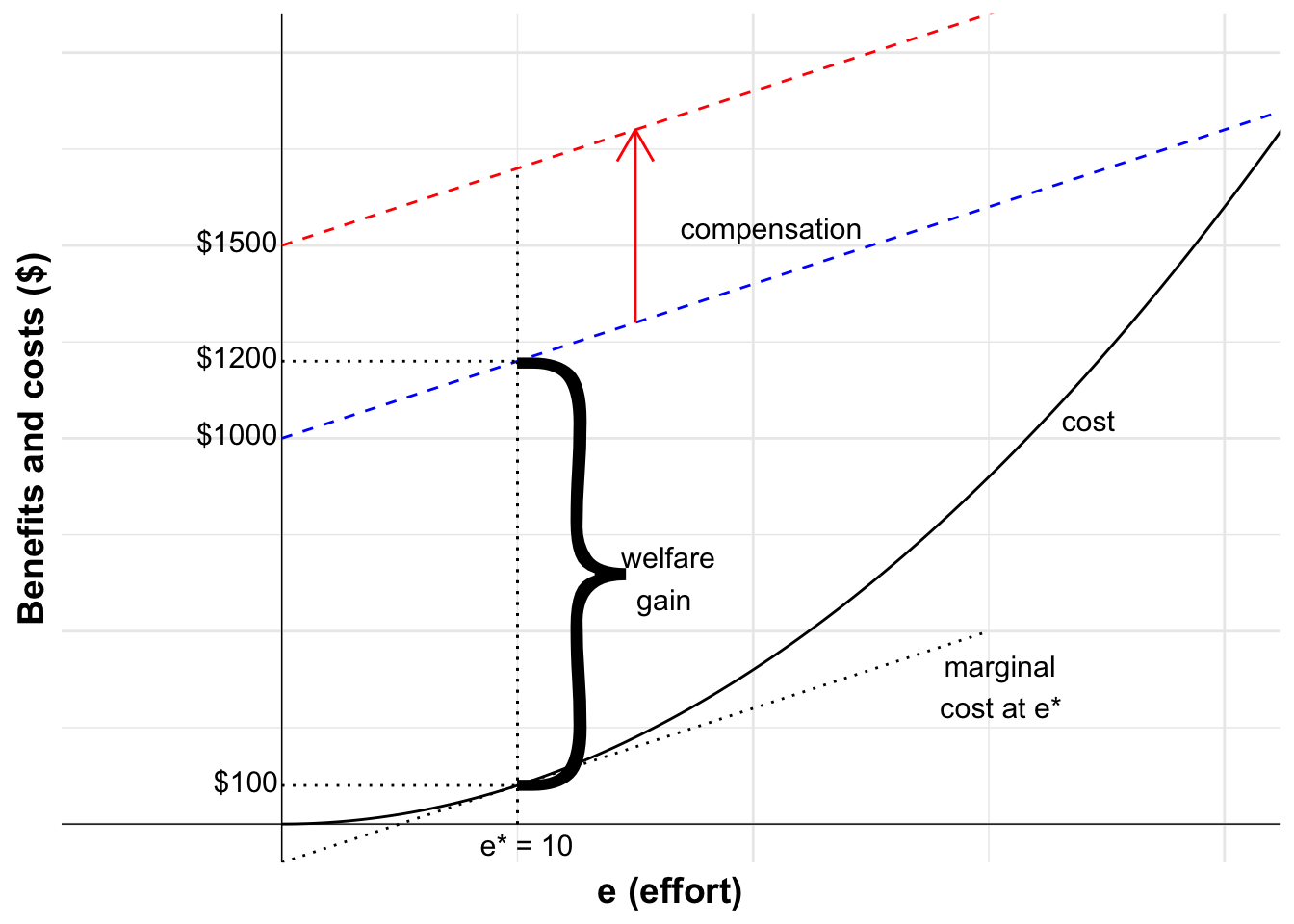
Mathematically, we can show this as follows. Suppose the firm increases the fixed wage to $1500. The utility function is therefore:
U=1500+20e+0.2\mu-e^2
The first order condition with respect to e is:
U_e=20-2e=0 \\[6pt]
e^*=10
This gives us the optimal effort level of 10, the same as for the lower fixed wage. Erica’s total compensation increases to $1700. The plot below illustrates this.
Code
ericaPlot3+#Add the compensation line starting at the base paygeom_segment(aes(x =0, y =1500, xend =100, yend =3500), linetype ="dashed", color ="red")+#Add vertical line indicating equilibirum stays the sameannotate("segment", x = estar, xend = estar, y =0, yend =compensation(estar)+500, linewidth =0.5, colour ="black", linetype="dotted")+#Add red vertical line with arrow between the two compensation lines indicating increaseannotate("segment", x =15, xend =15, y =compensation(15), yend =compensation(15)+500, arrow =arrow(type ="open", angle =30, length =unit(0.5, "centimeters")), colour ="red")+#add label for new higher fixed wageannotate("text", x =-2, y =1500, label ="$1500", size =4)+#add vertical lines with arrows to indicate welfare gaingeom_segment(aes(x = estar, xend = estar, y =cost_erica(estar), yend =compensation(estar)+500), colour ="black", linetype ="dashed", arrow =arrow(type ="closed", length =unit(0.15, "inches")))+geom_segment(aes(x = estar, xend = estar, y =compensation(estar), yend =cost_erica(estar)), colour ="black", linetype ="dashed", arrow =arrow(type ="closed", length =unit(0.15, "inches")))+annotate("text", x = estar +3.7, y = (cost_erica(estar) +compensation(estar)+500) /2, label ="welfare gain", size =4, colour ="black")+# Add line indicating new compensation equilibrium plus labels for new higher equilibrium compensationannotate("segment", x =0, y =compensation(estar)+500, xend = estar, yend =compensation(estar)+500, linewidth =0.5, colour ="black", linetype="dotted")+annotate("text", x =-2, y =compensation(estar)+500, label ="$1700", size =4)+# Add label to compensation lineannotate("text", x =14, y =1900, label ="compensation", size =4, color ="red")
Figure 5.7: Increasing the fixed wage with unobservable effort
5.2.2.2 Increasing the share of output
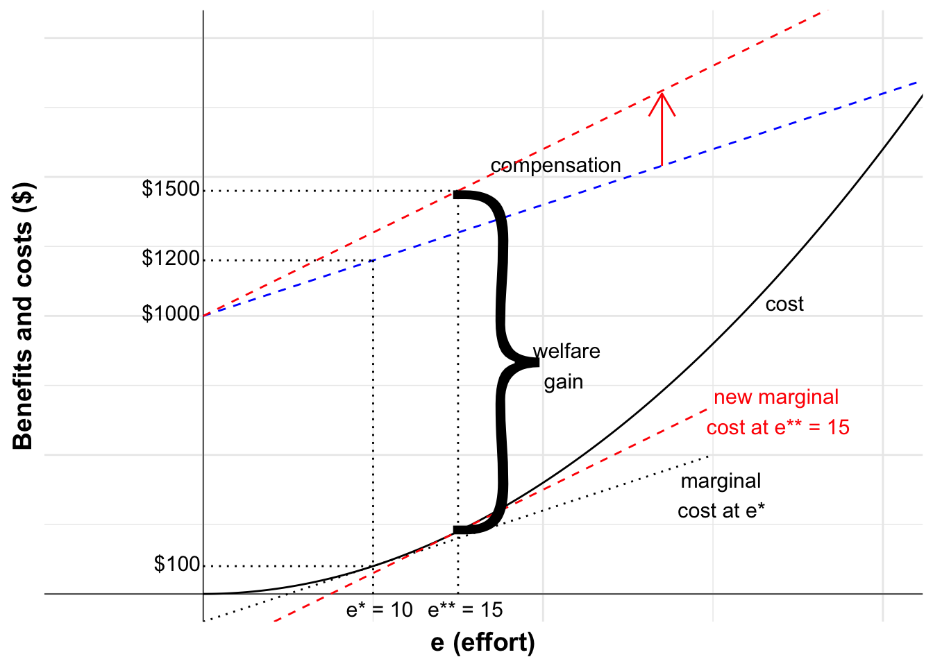
A change in \beta changes the optimal effort level. The optimal choice of effort is increased as the marginal benefit of effort is increased.
Mathematically, we can show this as follows. Suppose the firm increases the share of output to 0.3. The utility function is therefore:
U=1000+30e+0.2\mu-e^2
The first order condition with respect to e is:
U_e=30-2e=0 \\[6pt]
e^*=15
This gives us a higher optimal effort level of 15. The plot below illustrates this.
Code
ericaPlot3+#Add the compensation line starting at the base paygeom_segment(aes(x =0, y =1000, xend =100, yend =4000), linetype ="dashed", color ="red")+#add a tangent to the cost curve at e** and a label "new marginal cost"annotate("segment", x =0, xend =30, y =-225, yend =675, linewidth =0.5, colour ="red", linetype="dashed")+annotate("text", x =33, y =700, label ="new marginal\ncost at e**", size =4, color="red")+#Add vertical line at new higher equibrium effortannotate("segment", x =15, xend =15, y =0, yend =1450, linewidth =0.5, colour ="black", linetype="dotted")+annotate("text", x =15, y =-50, label ="e** = 15", size =4)+#Add red vertical line with arrow between the two compensation lines indicating increaseannotate("segment", x =27, xend =27, y =compensation(27), yend =compensation3(27), arrow =arrow(type ="open", angle =30, length =unit(0.5, "centimeters")), colour ="red")+#add #add vertical lines with arrows to indicate welfare gaingeom_segment(aes(x =15, xend =15, y =cost_erica(15), yend =compensation3(15)), colour ="black", linetype ="dashed", arrow =arrow(type ="closed", length =unit(0.15, "inches")))+geom_segment(aes(x =15, xend =15, y =compensation3(15), yend =cost_erica(15)), colour ="black", linetype ="dashed", arrow =arrow(type ="closed", length =unit(0.15, "inches")))+annotate("text", x =18, y = (cost_erica(15) +compensation3(15)) /2, label ="welfare\ngain", size =4)+# Add line indicating new compensation equilibrium plus label for new higher equilibrium compensationannotate("segment", x =0, y =1000+15*30, xend =15, yend =1000+15*30, linewidth =0.5, colour ="black", linetype="dotted")+annotate("text", x =0, y =1000+15*30, label ="$1500", size =4, hjust =1.05, vjust =0.3)+# add label to compensation lineannotate("text", x =19, y =1750, label ="compensation", size =4, color ="red")
Figure 5.8: Increasing the output share with unobservable effort
5.3 Optimal incentive schemes
Given this principle-agent problem, what should a firm do? It will try to maximise profit.
To do this, first it needs to ensure that the reservation level of utility is met, otherwise the individual will not work for the firm. One way to do this is to adjust the base pay, w_0, to ensure this is the case.
Then the firm needs to induce effort. It will want to set \beta at the right level. But this comes at a cost to the firm. With greater reward for effort we would expect that Agent B will work harder - this should lead to higher payments for the firm. But with higher \beta Agent B is exposed to increased risk. For a risk averse worker this will generally mean that Agent B will need to be compensated more so that they are willing to bear the higher risk.
What does all this mean? The following five factors favour high incentive pay:
A strong relationship between the employee’s effort and output, meaning the benefits of motivating effort are high
The employee has low risk aversion, as a person with high risk aversion will require higher compensation to bear the risk. In Erica’s example, we specified that she was rislk neutral. If she were risk averse, the possibility of large random shocks, even if independent of effort, would require a higher share of output to be paid to her to induce her to accept the contract.
A low level of risk that is beyond the control of the employee (\sigma^2), as output is then primarily a function of greater effort. This is the converse of the previous point.
High sensitivity to increased incentives (e.g the cost of effort is not so high as to prevent a response to the incentive)